Search results for 'q'
-
DBM 449 lab 2 OEM Query optimization
$20.00In this lab we will focus on several common performance tuning issues that one might encounter while working with a database. You will need to refer to both your text book and the lecture material for this week for examples and direction to complete this lab.
To record your work for this lab use the LAB2_Report.doc found in Doc Sharing. As in your first lab you will need to copy/paste your SQL statements and results from SQL*Plus into this document. This will be the main document you submit to the Drop Box for Week 2.L A B S T E P S
STEP 1: Examine Query Optimization using OEMOracle Enterprise Manager (OEM) provides a graphical tool for query optimization. The tables that you will be using in this lab are the same ones that were created in the first lab in the DBM449_USER schema.
- Start OEM via Citrix iLab. If you need help or instructions on how to do this you can refer to the How_to_use_OEM_in_Citrix iLab.pdf file associated with this link.
- Select Database Tools icon from the vertical tool bar and Select SQL Scratchpad icon from the expanded tool bar. If you need help or instructions on how to do this your can refer to theExecuting_and_Analyzing_Queries_in_OEM.pdf file associated with this link.
- Write a SQL statement to query all data from table COURSE (you will need to connect as the DBM449_USER). Click on Execute. Take a screen shot that shows the results and paste that into the lab document.
- Click on Explain Plan. Take screen shot of the results and past that into the lab document.
- Write a comment how this query is executed.
- Write a SQL statement to query the course_name, client_name and grade from the COURSE, COURSE_ACTIVITY and CLIENT tables and order the results by course name, and within the same course by client name.
- Click on Explain Plan. Take screen shot of the results and past that into the lab document.
- Exit out of OEM at this point.
- Write a comment on how this query is executed.
STEP 2: Examine Query Optimization using SQL*Plus
In this portion of the lab we are going to use SQL*Plus to replicate what we did in Step one using OEM. At the end of this part of the lab you will be asked to compare the results between the processes.
- Before you can analyze an SQL statement in SQL*Plus you first need to create a Plan Table that will hold the results of your analysis. To do this you will need to download the UTLXPLAN.SQL file associated with this link and run this script in an SQL*Plus session while logged in as the DBM449_USER user. Once the script has completed then execute a DESC command on the PLAN_TABLE.
- Again you are going to write a SQL statement to query all data from table COURSE. Remember to make the modifications to the query so that it will utilize the plan table that you just created.
- Now write the query that will create a results table similar to the one below by using the DBMS_XPLAN procedure.
PLAN_TABLE_OUTPUT
Plan hash value: 1263998123
Id Operation Name Rows Bytes Cost (%CPU) Time
0 SELECT STATEMENT 5 345 3 (0) 00:00:01
1 TABLE ACCESSFULL COURSE 5 345 3 (0) 00:00:01
Note
PLAN_TABLE_OUTPUT
- dynamic spamling used for this statement- Now execute the second query you used in Step 1 and then show the results in the plan table for that query. HINT: Before you run your second query you will need to delete the contents of the plan table so that you will get a clean analysis.
- Write a short paragraph comparing the output from OEM to the output from the EXPLAIN PLAN process you just ran. Be sure to copy/paste all of the queries and results set from this step into the lab report section for this step.
STEP 3: Dealing With Chained Rows
In this portion of the lab we are going to create a new table and then manipulate some data to generate a series of chained rows within the table. After you have generated this problem then we are going to go through the process of correcting the problem and tuning the table so that the chained rows are gone. The process is a little tricky and is going to require you to think through your approach to some of the SQL. Remember that every table has a hidden column named ROWID that is created implicitly by the system when the table is created. This column can be queried just like any other column. You will need this information in step 6 of this part of the lab.
- For this part of the lab you will need to create a new user named GEORGE. You can determine your own password but you want to make sure that the default tablespace is USERS and the temporary tablespace is TEMP. Grant both the connect and resource rolls to the new user and then log in to create a session for the new user GEORGE.
- Once logged in to the new user then write the SQL to create a new table using the given column information and storage parameters listed below. NOTE: the parameters have been chosen intentionally so please do not change them.
Table name: NEWTAB
Columns: Prod_id NUMBER
Prod_desc VARCHAR2(30)
List_price NUMBER(10,2)
Date_last_upd DATETablespace: USERS
PCTFREE 10
PCTUSED 90
Initial and Next extents: 1K
MinExtents 1
MaxExtents 121
PCTINCREASE 0- Next, you will need to download both the UTLCHAIN.SQL and LAB2_FILL_NEWTAB.SQL scripts from the links shown. First run the UTLCHAIN script in your SQL*Plus session and then run the LAB2_FILL_TAB script. Be sure that you run them in the order just described.
- Now execute the ANALYZE command on the table NEWTAB to gather any chained rows. HINT: refer back to the lecture material for this week and your text book.
- Write and execute the query that will list the owner_name, table_name and head_rowid columns from the CHAINED_ROWS table. You will have approximately 200+ rows in your result set so please do not copy/paste all of them into the lab report. You only need the first 10 or 15 rows as a representation of what was returned.
- Now you need to go through the steps of getting rid of all the chained rows using these steps.
- You can create your temporary table to hold the chained rows of the NEWTAB table as a select statement based on the existing table. HINT: CREATE TABLE NEWTAB_TEMP AS SELECT * FROM NEWTAB.... You want to be sure that you only pull data from the existing table that matches the data in the CHANED_ROW table. To assure this you will need a WHERE clause to pull only this records with a HEAD_ROWID value in the CHAINED_ROWS table that matches a ROWID value for the NEWTAB table.
- Now you need to delete the chained rows from the NEWTAB table. To accomplish this you will need a subquery that pulls the HEADROW_ID value from the CHAINED_ROWS table to match against the ROWID value in the NEWTAB table. The number of rows deleted should be the same as the number that you retrieved in the query for part 5 of this section.
- Now write an insert statement that will insert all of the rows of data in the temporary table that you created above into the NEWTAB table. Be sure that you explicitly define the rows that you are pulling data from in the NEWTAB_TEMP table.
- Next, write and execute the statement that will TRUNCATE the chained_rows table.
- Now run the same ANALYZE statement you did in step 4 and then the query you did in part 5 above. This time you should get a return message stating no rows selected.
Be sure that you copy/paste all of the above SQL code and returned results sets and messages into the appropriate place in the Lab Report for this week.
Deliverables
Learn More
What is Due
Submit your completed Lab 2 Report to the Dropbox as stated below. Your report should contain copies of each query and result set outlined in the lab along with the requested explanation of whether or not it satisfied the business requirement outlined for that particular section of the lab.
-

DBM 449 Lab 3 Distributed Database
$20.00L A B O V E R V I E W
Scenario/Summary
To the end user working with databases distributed through out a company's network is not different than working with multiple tables within a single database. The fact that the different databases exist in other locations should be totally transparent to the user. For this lab we are going to take on the roll of a database administrator in a company that has three regional offices in the country. You work in the central regional office, but there is also a West Coast Region located in Seattle and an East Coast Region located in Miami. Your roll is to gather report information from the other two regions.For this lab you are going to work with three different databases. You already have your own database instance. You will also be working with the a database named SEATTLE representing the West Coast Region and a database named MIAMI representing the East Coast Region. Login information for these two additional database instances is as follows:
SEATTLE: Userid - seattle_user
Password - seattle
Host String - seattleMIAMI: Userid - miami_user
Password - miami
Host String - miamiTo record your work for this lab use the LAB3_Report.doc found in Doc Sharing. As in your previous labs you will need to copy/paste your SQL statements and results from SQL*Plus into this document. This will be the main document you submit to the Drop Box for Week 3.
L A B S T E P S
STEP 1: Setting up Your Environment- Be sure you are connected to the DBM449_USER schema that was created in lab 1.
- To begin this lab you will need to download the LAB3_DEPTS.SQL script file associated with the link and run the script in your DBM449_USER schema of your database instance. This script contains a single table and that you will be using to help pull data from each of the other two database instances. Notice that the DEPTNO column in this table is the PRIMARY KEY column and can be used to reference or link to the DEPTNO column in the other two database employee tables.
- Now you need to create a couple of private database links that will allow you to connect to your other two regional databases. To accomplish this use the connection information listed above in the Lab Overview section. Name your links using your database instance name together with the region name as the name for the link. Separate the two with an underscore (example - DB1000_SEATTLE).
- After creating both of your database links, query the USER_DB_LINKS view in the data dictionary to retrieve information about your database links. The output from your query should look similar to what you see below. You will need to set your linesize to 132 and format the DB_LINK and HOST columns to be only 25 bytes wide to get the same format that you see.
DB_LINK USERNAME HOST CREATED
------------------------- ------------------------------ ------------------------- ---------
DB1000_MIAMI MIAMI_USER miami 09-DEC-08STEP 2: Testing your Database Links
Each of your remote databases has an employee data table. The tables are named SEATTLE_EMP and MIAMI_EMP respective to the database they are in. Using the appropriate database link, query each of the two tables to retrieve the employee number, name, job function, and salary. (HINT: you can issue a DESC command on each of the distributed tables to find out the actual column names just like you would for a table in your own instance.STEP 3: Connecting Data in the Seattle Database
Write a query that will retrieve all employees from the Seattle region who are salespeople working in the marketing department. Show the employee number, name, job function, salary, and department name (HINT: The department name is in the DEPT table) in the result set.STEP 4: Connecting Data in the Miami Database
Write a query that will retrieve all employees from the Miami region who work in the accounting department. Show the employee number, name, job function, salary, and department name (HINT: The department name is in the DEPT table) in the results set.STEP 5: Connecting Data in all Three Databases
Now we need to increase our report. Write a query that will retrieve employees from both the Seattle and Miami regions who work in sales. Show the employee number, employee name, job function, salary and location name in the result set (HINT: The location name is in the DEPT table).STEP 6: Improving Data Retrieval from all Three Databases
Writing queries like the ones above can be fairly cumbersome. It would be much better to be able to pull this type of data as though it was coming from a single table, and in fact this can be done by creating a view.- Using the query written above as a guide, write and execute the SQL statement that will create a view that will show all employees in both the Seattle and Miami regions (you can use your own naming convention for the view name). Show all the employee number, name, job, salary, commission, department number and location name for each employee (HINT: The location name is in the DEPT table).
- Now write a query that will retrieve all the data from the view just created.
Deliverables
Learn More
Submit your completed Lab 3 Report to the Dropbox. Your report should contain copies of each query and result set outlined in the lab along with the requested explanation of whether or not it satisfied the business requirement outlined for that particular section of the lab. -
DBM 449 Lab 4 Oracle Object type
$20.00L A B O V E R V I E W
Scenario/Summary
For this lab you will begin by using the same set of tables that you used for Lab 1 so be sure that you are connected to Oracle as the DBM449_USER user. The objective of this lab will be to create a series of object-relational tables using the SQL*Plus editor that will allow data to be stored in a more "real-world" format. Data for your new tables can be found in the file Lab4_data.txt associated with this link. You will need to manipulate the data in various ways, but the file will give you access to the raw data to use.
To record your work for this lab use the LAB4_Report.doc found in Doc Sharing. As in your previous labs you will need to copy/paste your SQL statements and results from SQL*Plus into this document. This will be the main document you submit to the Drop Box for Week 4.L A B S T E P S
STEP 1: Create a table with a column data type
Modify the design of the COURSE table created in iLab 1 to incorporate the use of the column abstract data type.- Write and execute the SQL to create a single object type called COURSE_OBJ1 that contains both the attributes course code and course name. Remember that with abstract objects you must use the / after the CREATE statement to execute it.
- Next, write and execute the SQL to create a table called NEW_COURSE1 that contains COURSE_OBJ1 along with the original attributes from the original COURSE table. Keep in mind what attributes the new object type COURSE_OBJ1 contains. Your table should have a total of 4 individual columns when finished.
- Using the data from the LAB4_DATA file create and execute the insert statements to load the new table NEW_COURSE1. SUGGESTION: Using the Lab4_data file create a script file of your insert statements and then run the script file. Remember that you will need enclose some of the data in single quotes depending on if it is character, date, or numeric data.
- Run DESCRIBE command to describe structure of table NEW_COURSE1.
- SET DESCRIBE DEPTH 2 and run DESCRIBE NEW_COURSE1 again.
- Execute a SELECT statement to query the data from the new table (DO NOT use a SELECT * type query). Use the COLUMN column_name FORMAT A## session command to format columns within the table to keep the result set data from wrapping around. Be sure that you properly display data inside the object column. (HINT: When querying attributes of an abstract data type, you must use a correlation variable for the table.)
STEP 2: Create an object table with a row data type
Create a second COURSE table, this time as an object table using the row abstract data type.- Write and execute the SQL to create an object called COURSE_OBJ2 that contains the attributes course code, course name, course date, instructor, and location.
- Write and execute the SQL to create a table called NEW_COURSE2 with a single column defined using the COURSE_OBJ2 object.
- Using the data from the LAB4_DATA file create execute the insert statements to load the new table NEW_COURSE2.
- Execute a SELECT statement to query the data from the new table (DO NOT use a SELECT * type query).
STEP 3: Create a Varying Array
Modify the design of the CLIENT table created in iLab 1 to incorporate the use of the Varying Array.- Write and execute the SQL to create a Varying Array to represent the phone contact information for the client (up to 3 phone numbers). Name the varying array as PHONE_LIST.
- Write and execute the SQL to create a table called NEW_CLIENT that contains the attributes that the original CLIENT table contained plus the phone list array.
- Using the data from the LAB4_DATA file create execute the insert statements to load the new table NEW_CLIENT.
- Execute a SELECT statement to query the data from the CLIENT_NO and CLIENT_NAME columns along with the data in the column containing the phone number Varray (You cannot use a SELECT * type query for this step).
Deliverables
Submit your completed Lab 4 Report to the Dropbox. Your report should contain copies of each query and result set outlined in the lab along with the requested explanation of whether or not it satisfied the business requirement outlined for that particular section of the lab.
Learn More -
DBM 449 Lab 5 Audit and Profile Management
$20.00In your lab for this week you are going to work with three different areas and processes within the Oracle Database that can be used to control data security. Each of these three processes has its own distinctive application to providing levels of security. In each case the individual processes deal with either limiting a users access to the database, limiting access to processes within the database, or keeping track of what the user is doing while in the database.
For the lab you will be using the SCOTT user which is already created in your instance. In Step 4 you will also be asked to shutdown you instance, make some edits to the init.ora file for your instance and then restart the instance. If you are not comfortable with this process which was first introduced to you in DBM438 the refer to the iLab Manual found in week 1 for guidance.
To record your work for this lab use the LAB5_Report.doc found in Doc Sharing. As in your previous labs you will need to copy/paste your SQL statements and results from SQL*Plus into this document. This will be the main document you submit to the Dropbox for Week 5.
LAB STEPS
STEP 1: Define a New Profile
Oracle provides the ability to set expirations, limit the reuse, and define the complexity of passwords. In addition, accounts can be locked if the password is entered incorrectly too many times. In this section of the lab we are going to create a custom profile that will then be applied to the SCOTT user.
- To begin, log into your instance as the SYS user.
- Write SQL script that will create a new profile named DBM449_SCOTT_PROFILE that will do the following:
- Limit the number of failed login attempts to 3 in a row.
- Limit the overall connection time to 10 hours (we will give him a little leeway incase he has to work overtime).
- Allow a session to be idle no more than 1 hour.
- Change the password every 60 days.
- Allow the user 3 days to change the password after it expires.
- Not allow a previous password be reused before there have been three password changes.
- Execute your pfile script and verify that the profile has been created by running a query against the DBA_PROFILES view in the data dictionary. Limit your output to ONLY the DBM449_SCOTT_PROFILE parameters.
Be sure to copy/paste your script and results sets output to the appropriate section in the Lab5_report document.
STEP 2: Testing the New Profile
Now that we have a new profile for the SCOTT user we need to verify that it works properly. For obvious reasons there are going to be parts of the profile that we cannot test within the confines of this lab due to time constraints, but we can test to verify that the SCOTT user is being controlled by the profile.
- The first thing we need to do is assign the profile to the SCOTT user. While still logged into your instance as the SYS user write and execute the SQL command that will assign the new SBM449_SCOTT_PROFILE profile to the SCOTT user.
- Now log into SCOTT (password is TIGER). Remember that you must supply the database instance name when logging in from the SQL> prompt just as you do when using the login window, i.e. CONN SCOTT/TIGER@DB####.WORLD.
- There are several things that we can test related to the logging in and changing a password so here we go.
- You should now be successfully connect to the SCOTT user. Write the connect command again on this time use an incorrect password. NOTE: you should get a warning message stating that you are no longer connected to Oracle. That is fine, just keep trying to log in.
- Repeat the above process until you get the ORA-28000: the account is locked error which will indicate that the profile is working here.
- At this point we need to get the account unlocked so you will need to login to your instance as the SYS user and unlock the SCOTT account BUT DO NOT LOG BACK INTO THE SCOTT USER YET.
- Now we can test the password reuse parameter. To do this we must EXPIRE the current password. Write and execute the SQL command to expire the password for the SCOTT user.
- Now log back into the SCOTT user. You should receive a message stating that the password has expired (ORA-28001: the password has expired) and then prompting you to change the password.
- Try to reuse the TIGER password. You should receive the following - ORA-28007: the password cannot be reused.
- Now log into the SCOTT user again and this time change the password to LION to complete this step of the lab.
Be sure to copy/paste your script and results sets output to the appropriate section in the Lab5_report document.
STEP 3: Using the PRODUCT_USER_PROFILE table
As the owner of a schema a user has certain inherited privileges that would allow the user to pass access to his/her own objects on to other users. Often times this can open up data to scrutiny by individuals who probably do not need to have access to it. These types of decisions should always be made by the DBA in charge of the database. One mechanism the DBA has to keeping users from using these inherited privileges is by excluding those commands using the PRODUCT_USER_PROFILE (PUP) table. In this section of the lab we are going to do this to the SCOTT user by setting up the scenario that will prohibit him from giving the user GEORGE (created in lab 2) access to the EMP table.
- For this section and remainder of the lab you must have the PRODUCT_USER_PROFILE successfully loaded and accessible in your instance. The creation of this profile was one of the first things done back in Lab 1 when you ran the PUPBLD.SQL script. If you are getting an error message stating "Error accessing PRODUCT_USER_PROFILE" when you log in as the DBM449_USER or the SCOTT user then this profile is not successfully installed. Work with your instructor to figure out why your script from Lab 1 did not work correctly. Until this is resolved you will not be able to complete the remainder of the lab.
- If you have the PRODUCT_USER_PROFILE successfully working then log in to your database instance as the SYS user.
- Now we need to limit SCOTT from being able to use the GRANT command.
- Insert the proper values into the PRODUCT_USER_PROFILE table that will keep the SCOTT user from using the GRANT command. Remember that some of the values in your insert statement must be in upper case and some will need to be in mixed case. Once you have done this then query the table to verify the insert (REMEMBER: you cannot query the table as the SYS user, only as the SYSTEM user).
- Now we need to test our above settings and make sure they are working.
- Connect to the SCOTT user (remember that you changed the password to LION).
- Write and execute the statement that would GRANT the user GEORGE the ability to write a select statement and see the data in the EMP table owned by SCOTT. You should receive the following message - SP2-0544: Command "grant" disabled in Product User Profile.
- This verifies that you have now disabled the ability of the SCOTT user to allow another user to access any of the data in his schema.
Be sure to copy/paste your script and results sets output to the appropriate section in the Lab5_report document.
STEP 4: Setting up the Database to use Auditing
Being able to audit what, when and where people are doing things in the database can be a very enlightening thing for a DBA. It can also be a very important tool in working with Data Security. Oracle provides the ability to do various types of auditing, but it takes some special setting up of the environment for this to work. In this step we are going to make the necessary adjustments to the current Oracle instance so that we can enable auditing and make some tests. If you need to review the processes to be used here then refer to the iLab Manual in week 1.
- First you need to make sure that you are logged into your instance as the SYS user.
- At this point issue a SHUTDOWN IMMEDIATE command to shut down you database instance.
- Once the instance is shut down you need to go into your Citrix Windows Explorer application, find your database instance set of directory folders, drill down to the pfile directory folder and open your init.ora file found in that folder.
- Under the section titled "Security and Auditing" you need to add the parameter AUDIT_TRAIL and set the parameter to DB_EXTENDED. This will allow the SQL_TEXT column of the DBA_AUDIT_OBJECT view to be populated. Save and close the file and then go back to your SQL*Plus session.
- Now using the init.ora file, start your instance back up to an OPEN status. You can do this by issuing a STARTUP PFILE= statement and pointing to your init.ora file.
- Once you have completed this process you are ready to begin setting up the database to audit some activity.
Be sure to copy/paste your script and results sets output to the appropriate section in the Lab5_report document.
STEP 5: Creating an Audit Trail
Oracle permits audit trails to be generated for session login attempts, access to objects, and activity performed on objects. Again using the SCOTT user we are going to set up several scenarios for auditing what SCOTT does while in a session. NOTE: if you need to work through this process several times you can delete the values in the AUD$ base table by issuing the TRUNCATE TABLE AUD$ command while logged in as the SYS user.
- Make sure that you are connected as user SYS.
- Display value of the parameter AUDIT_TRAIL. For the VALUE column you should have a value of DB_EXTENDED.
- Now we can set up auditing to track what goes on in the database.
- Write SQL statements to audit successful and unsuccessful login attempts by SCOTT.
- Write SQL statement to audit any successful INSERT, UPDATE or DELETE performed on table DEPT in scott's schema.
- Now we need to test the audits to verify that they work.
- Log into the SCOTT user (remember that the password is LION) and perform the following:
- write and execute an UPDATE statement that will change the value in the LOC column of the DEPT table to MIAMI where the DEPTNO value is 10. Be sure to issue a COMMIT.
- Write and execute the INSERT statement that will in insert the following values into DEPT - (50, 'LEGAL', 'HOUSTON'). Be sure to issue a COMMIT.
- Write and execute the DELETE statement that will delete the row from the DEPT table that was just inserted in the step above. Again, be sure to issue a COMMIT.
- Try to reconnect to the SCOTT user with an invalid password.
- Now connect back to the SYS user.
Now we need to see if our auditing worked.
- While logged into your instance as the SYS user, query the DBA_AUDIT_OBJECT view of the data dictionary for the user name of the account (Not the OS), the object owner, the object name, the action name and the SQL command (text) from the DBA_AUDIT_OBJECT view in the Data Dictionary.
- Did you notice that the entries for successful logon and unsuccessful logon attempts were not there. Now query the user name, action name and return code values in the DBA_AUDIT_SESSION view. You should find that information here.
Be sure to copy/paste your script and results sets output to the appropriate section in the Lab5_report document.
Deliverables
Submit your completed Lab 5 Report to the Dropbox. Your report should contain copies of each query and result set outlined in the lab along with the requested explanation of whether or not it satisfied the business requirement outlined for that particular section of the lab.
Learn More -
DBM 449 Lab 6 SQL Analytical Extensions and Materialized Views
$20.00For the lab this week we are going to look at how the ROLLUP and CUBE extensions available in SQL can be used to create query result sets that have more than one dimension to them. Both of these extensions are used in conjunction with the GROUP BY clause and allow for a much more broad look at the data.
The first thing you will do for this lab is download the lab6_create.sql file and run the file in your database instance. This file will log into the DBM449_USER and then create and populate a set of tables that will be used for this lab. Instructions for this are outlined in Step 1.
To record your work for this lab use the LAB6_Report.doc found in Doc Sharing. As in your previous labs you will need to copy/paste your SQL statements and results from SQL*Plus into this document. This will be the main document you submit to the Dropbox for Week 6.
LAB STEPS
STEP 1: Setting up Your Instance
For this lab you will be using a different user and set of tables than you have used so far for other labs. To set up your instance you will need to do the following.
- Download the lab6_create.sql file associated with the link to either the C drive on your computer or the F drive in your Citrix account.
- Open up the file and edit the login information at the top for the new user that is being created. You will need to replace the @ORACLE piece with the specifics for your instance name. DO NOT include AS SYSDBA after the name of your instance for this login.
- Now log into your instance as the SYS user. Run the script. The script is too long to copy/paste it into your SQL*Plus session so you should run the script using the @ sign from the SQL> prompt.
- Once the script has finished running then issue a SELECT * FROM TAB; sql statement. The result set will have tables from other labs as well but you want to make sure that you see the following tables listed.
TNAME TABTYPE CLUSTERID
------------------------------ ------- ----------
SUPPLIER TABLE
PRODUCT TABLE
DISTRICT TABLE
CUSTOMER TABLE
TIME TABLE
SALES TABLESTEP 2: Using the ROLLUP Extension
In this section of the lab you are going to create a sales report that will show a supplier code, product code and the total sales for each product based on unit price times a quantity. More importantly the column that shows the total sales will also show a grand total for the supplier as well as a grand total over all (this will be the last row of data shown). To do this you will use the ROLLUP extension as part of the GROUP BY clause in the query. Use aliases for the column names so that the output columns in the result set look like the following.
SUPPLIER CODE PRODUCT TOTAL SALES
------------- ---------- -----------For this report you are going to use the SALES, PRODUCT and SUPPLIER tables. You should be able to write your query using NATURAL JOIN but if you feel more comfortable using a traditional JOIN method that will work just as well. When finished you should have a total of 16 rows in your report and the grand total amount should show 2810.74.
Be sure to copy your SQL code and the result set produced and paste it into the appropriate place in the LAB6_REPORT.
STEP 3: Using the CUBE Extension
In this section of the lab you are going to create a sales report that will show a month code, product code and the total sales for each product based on unit price times a quantity. In this report the column that shows the total sales will also show a subtotal for each month (in this case representing a quarter) . Following the monthly totals for each product and the subtotal by month then the report will list a total for each product sold during the period with a grand total for all sales during the period (this will be the last row of data shown). To do this you will use the CUBE extension as part of the GROUP BY clause in the query. Use aliases for the column names so that the output columns in the result set look like the following.
MONTH PRODUCT TOTAL SALES
---------- ---------- -----------For this report you are going to use the SALES, PRODUCT and TIME tables. You should be able to write your query using NATURAL JOIN but if you feel more comfortable using a traditional JOIN method that will work just as well. When finished you should have a grand total amount of 2810.74 (same total as in the step 2).
Be sure to copy your SQL code and the result set produced and paste it into the appropriate place in the LAB6_REPORT.
STEP 4: Materialized Views and View Logs
Materialized views, sometimes referred to as snapshots are a very important aspect of dealing with data when doing data mining or working with a data warehouse. Unlike regular views, a materialized view does not always automatically react to changes made in the base tables of the view. To help keep track of changes made to the base tables you must create what is call a Materialized View Log on each base table that will be used in the view. In this step of the lab we will do this.
For the Materialized View we are going to create we are going to use the TIME and the SALES tables. Before we can create the view you will need to create a Materialized View Log on each of these two tables that will keep track of the ROWID and Sequence and include new values that have been added to the base table.
Be sure to copy your SQL code and the result set produced and paste it into the appropriate place in the LAB6_REPORT.
STEP 5: Creating and Using the Materialized View
Now that we have our logs created we can progress on to the view itself. For this part of the lab you are going to create a Materialized View, demonstrate that the view works, insert a row of data into one of the base tables and then update the view. Finally, you will show that the new data is in the view. The following steps will help move you through this process.
- First, write the SQL CREATE statement that will create a Materialized View based on the following:
- Name the view SALESBYMONTH.
- Include clauses that will build the view immediately, completely refresh the view, and enable a query rewrite.
- For the columns of the view you want to show the YEAR, MONTH, PRODUCT CODE, a TOTAL SALES UNITS, and a TOTAL SALES.
- You will want to group the columns by year, month and product code respectively.
- Execute your script to create the view and then issue a SELECT * FROM SALESBYMONTH.
The output columns from your view should look similar to the following (use aliases to format the column headings) and you should have 18 rows in the result set.
YEAR MONTH PRODUCT CO UNITS SOLD SALES TOTAL
-------- ---------- ---------- ---------- -----------Now we are going to add some data and update the view. Because we have several derived columns in out view we will have to force the update as Oracle will not automatically update a view with this configuration.
- To begin with, insert the following data into the SALES table - (207, 110016, 'SM-18277',1,8.95).
- Now we are going to use a subprogram within the Oracle built in package DBMS_MVIEW. The REFRESH subprogram within this package will update our view so that we can see the new data.
- Write an SQL EXECUTE statement that will use the REFRESH procedure in the DBMS_MVIEW package (HINT: packagename.subprogram). The REFRESH subprogram accepts two parameters; the name of the materialized view to refresh, and either a 'c', 'f', or '?'. For the purposes of the lab use the 'c'. (you can refer back to pages 654-659 of the DBA Handbook readings for week 3).
- Execute your statement to update the view and then query the view once again.
You should now see that the row for units sold in month 10 for SM-18277 has increased from 3 to 4 and total sales amount has gone from 26.85 to 35.80.
Be sure to copy your SQL code and the result set produced and paste it into the appropriate place in the LAB6_REPORT.
Deliverables
Submit your completed Lab 6 Report to the Dropbox. Your report should contain copies of each query and result set outlined in the lab along with the requested explanation of whether or not it satisfied the business requirement outlined for that particular section of the lab.
Learn More -

CTS2437 Final Exam SQL Server Administration
$15.00CTS2437 – Final Exam Provide the SQL statements required to accomplish the following tasks. #1 (10 points) Create a database named FINAL_EXAM that you will then use for all remaining problems. #2 (20 points) Create the tables and appropriate constraints based on the following ER diagram. Use appropriate data types. Note that the size column should only accept S, M, or L. In addition the price column should have values greater than zero. All columns in both tables are required. Catgeory Product C #3 (5 points) Insert 3 rows in the Category table. The db is for a small shoe store, so use appropriate data for the description ( “Men”, “Women”, “Children”) #4 (5 points) Insert 3 Product records for each category in the product table. Use whatever data you see as appropriate. #5 (5 points) Use one statement to increase the price of all products in the Men category by 25%. #6 (5 points) Use one statement to delete all products for the Children category. #7 (10 points) Create and execute a view named EXAM_VIEW that shows all columns from both tables. Use an inner join. #8 (10 points) Create a database trigger named EXAM_TRIGGER that prevents a user from deleting a Product record on Tuesdays. Display an appropriate error message. Make sure to show that the trigger is working properly. #9 (10 points) Create a stored procedure named SP_EXAM that will be used to insert records into the Product table. Make sure to show that the procedure is working properly. #10 (5 points) Remove the EXAM_VIEW object from the database. #11 (5 points) Remove the SP_EXAM stored procedure from the database. #12 (5 points) Remove the EXAM_TRIGER database trigger from the database. #13 (5 points) Remove the FINAL_EXAM database. Learn More -
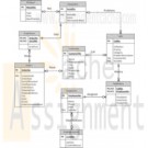
CTS2437 South Community College ERD and SQL script
$15.00South Community College (SCC) is structured like a typical community college. They have 3 semesters and a multitude of courses. Each course may have any number of sections in a given semester. For example, CTS2437 (SQL Server) may have one or more sections being taught in any given semester. SCC has 3 semesters (fall, spring, summer) which they refer to as A, B, and C. They refer to semesters by the year and the semester code. For example, fall 2011 would be referred to as 2011A. They need to keep track of students, courses, schedules, instructors, and grades earned in each course taken. They need a database to maintain these information. The student information would include the student name, address, phone#, and email. Students may have taken or are taking any number of courses. The grade earned for each course must also be maintained. The course information would include the course title and number of credits. Keep in mind that a given course may have many sections in any particular semester. SCC needs to maintain the instructor for each section in addition to the students and the grade they earned. The instructor information would include the instructor name, phone#, office#, and email address. South needs to maintain all courses that the instructor has taught or is currently teaching. Some of the requirements that SCC has requested in the database system include: • Student cannot register for the same section more than once. • A roaster of students can be produced for any given section. • GPA (Grade Point Average) can be generated for a student for any given semester, year, or entire school career. • GPA is calculated by adding up all of the grades earned (A=4, B=3, C=2, D=1, F=0) and dividing by the number of credits associated with the courses taken. • A transcript can be produced for a given student showing all courses taken and grades earned. Learn More -
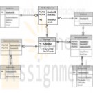
CIS 355 PCI Warranty Call Center Case ER Diagram
$15.00CIS 355 Term Project Part I For your term project, you are expected to design and implement a relational database to meet the requirements described in the PCI Warranty Call Center Case. Deliverables Part I - Project Design Document This document should have the following components: 1. A conceptual ER model/diagram of PCI’s data requirements. The diagram should include all relevant entities, attributes and relationships. For each entity, specify the identifier (primary key). Specify relationship names and cardinality constraints. Indicate which attributes are required, composite, multi- valued, and/or derived (Note: by default, an attribute is assumed to be optional, simple, single-valued and not derived). Indicate which entities are associative. Follow consistent naming conventions for entities and attributes. Use modeling/diagramming software to create the ER Diagram. 2. A list of the normalized relations (the logical model) and their attributes. For each relation, primary and foreign keys should be clearly indicated. Note: Use the format that we will be discussing in class for presenting your logical model. 3. A list of assumptions (if any) made about the information requirements presented in the case. Note: the assumptions should be reasonable and should not contradict the facts of the case. 4. A data dictionary that defines the metadata for the logical model. The data dictionary should include: the definition of each relation and attribute; the primary and foreign keys in each relation; attribute data types and lengths; and whether attributes are optional or required. Organize the data dictionary alphabetically by relation name. Assessment Part I deliverables will be evaluated based on the completeness and correctness/accuracy of the conceptual and logical data models, and of the supporting documentation (i.e., data dictionary, assumptions (if any)). If any of the deliverables are hand-drawn/written, your submission will not be graded. Submit the deliverables as one or more files. Include your name and title of the project on every page of the documents you submit. Learn More -
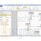
MIS582 iLab 2 Data Modeling Using Visio
$15.00MIS582 iLab 2: Data Modeling Using Visio
Learn More
iLAB OVERVIEW
Scenario and Summary
In this assignment, you will learn to create a physical database model in Visio from business requirements. To complete this assignment, you will need to be able to run Visio 2010, either through Citrix or installed on your workstation or laptop.
Deliverables
Name your Visio file using Lab2_, your first initial, and your last name (e.g., Lab2_JSmith.vsd). Create and save your database model in your Visio file.
iLAB STEPS
STEP 1:
Read the following business requirements closely to determine the entities and relationships needed to fulfill the requirements. The nouns in the paragraph will tell you the entities that will be needed. The verbs in the paragraph will help you determine the relationships between the entities.
Muscles Health Club Database Requirements:
The Muscles Health Club needs a database to keep track of its members, their personal trainers, and the fitness classes they are taking. Employees can act as personal trainers for members. However, only certified employees can act as personal trainers. A member can work with only one personal trainer at a time. Members can take multiple fitness classes. Fitness classes are taught by employees who can teach multiple classes. Fitness classes are taught in one of the classrooms at one of Muscles Health Club’s several locations. Each fitness classroom is designed for a different type of class (e.g., spinning, aerobics, water aerobics, weight training, etc.). It is necessary to track what fitness classes are being held in each of the different Muscles Health Club locations.
STEP 2:
• Run Visio 2010 either via Citrix or on your workstation.
• Click on the Software and Database Template group in the main window.
• Double-click on the Database Model Diagram Template to open a new file.
• Save the file with a name containing Lab2_, your first initial, and your last name as the file name (e.g., Lab2_JSmith.accdb). You will need to click the computer icon in the Save As window to see the different drives. Be sure to save the file to a local drive so it will be on your workstation.
STEP 3:
Add an entity for each entity you identified in the requirements.
• Drag the entity icon onto the drawing area in Visio.
• In the Database Properties window, add a physical name to identify it.
STEP 4:
For each entity, create a list of attributes you think would be useful to describe the entity.
• Select an entity in the drawing area of Visio.
• In the Database Properties window, select the Columns category.
• Use the table to add your attributes to the selected entities.
• Select one of the attributes to be the primary key (PK).
STEP 5:
Set the diagram to use crow’s feet notation.
• On the Database tab, in the Manage group, click Display Options.
• In the Database Document Option dialog, select the Relationship tab.
• Select the Crow’s Feet check box, and then click OK.
STEP 6:
Draw relationships between your entities.
• Drag the relationship icon onto a blank part of the drawing area.
• Connect the two ends to each of the two entities in the relationship. The parent entity must have a PK defined. The entity will be outlined in bold red lines when it connects to one end of the relationship.
STEP 7:
Set the cardinality of your relationships.
• Select a relationship line in the drawing area that is connecting two entities.
• In the Database Properties window, select the miscellaneous category.
• Select the cardinality for the selected relationship.
STEP 8:
When you are done, save the file on your local hard drive and upload it to the Course Project Drop box. Your file should have the following filename format: Lab2_FirstInitialLastName.vsd.
Submit your assignment to the Drop box located on the silver tab at the top of this page. -

MIS582 iLab 3 Database Construction Using Access
$15.00MIS582 iLab 3: Database Construction Using Access
iLAB OVERVIEW
Scenario and Summary
In this assignment, you will learn to create an Access database from a given ERD. To complete this assignment, you will need to be able to run Access 2010, either through Citrix or installed on your workstation or laptop.
Deliverables
Name your Access database file using Lab3_, your first initial, and your last name (e.g., Lab3_JSmith.accdb). Create and save your Access database file. When you are done, submit your database to the Course Project Dropbox.
iLAB STEPS
STEP 1:
Review the ERD below to understand the entities, attributes, primary keys, and relationships that you will create in your Access database.STEP 2:
• Run Access 2010, either via Citrix or from Visio 2010 installed on your workstation.
• Select the blank database icon in the main window.
• Save the file with a name containing Lab3_, your first initial, and your last name (e.g., Lab3_JSmith.accdb). In Citrix, you will need to click the computer icon in the Save As window to see the different drives. Be sure to save the file to a local drive so it will be on your workstation.
See the tutorials above for instructions on how to perform the following steps in Access 2010.STEP 3:
Learn More
Add tables to the Access database.
• Add a table for each entity listed in the provided ERD diagram.
• Add a column for each attribute listed in the provided ERD diagram.
• Select a primary key for each table as indicated in the provided ERD diagram.
STEP 4:
For every column in every table, update the data type as needed to enforce the domain constraints of the data.
• Dates should have a date data type.
• Surrogate keys should be autonumbered.
• Numeric data should have a numeric data type.
• Character data should have a character data type.
STEP 5:
Draw relationships between your entities.
• Selection Relationships under Database Tools. Move all your tables into the Relationship window by dragging them in or by using the Show Tables pop-up window.
• Second item
o Add the relationship between the tables in your database.
o Enable referential integrity on the relationship.
o Enable cascade updates on the relationship.
STEP 6:
Add at least two rows of data to each table in your database. Use any values you like for each of the columns. Remember that you must add data to parent tables before adding data to child tables, because referential integrity is enabled.
STEP 7:
Set the following column constraints in your database.
• Student first and last name cannot be a null value.
• Course credit hours must be between one and four.
• Course name must be unique and cannot be a null value.
• Instructor first and last name cannot be a null value.
• Grade must be one of these values: A, B, C, D, F, I, W, or E. W signifies withdrawn and E signifies enrolled.
STEP 8:
When you are done, save the file on your local hard drive and upload it to the Course Project Dropbox. Your file should have the following filename format: Lab3_FirstInitialLastName.accdb.
For instructions on how to copy files between the Citrix server and your local machine, watch the iLab tutorial, Copying Files from Citrix, located in the iLab menu tab under Course Home.
Note!
Submit your assignment to the Dropbox located on the silver tab at the top of this page.

You have no items in your shopping cart.
